First Attempt at Modeling Crime in Chicago

In my last post, I showed how to use the Socrata Open Data API (SODA) to download the data of the crimes reported in Chicago, how to plot the locations, and how to count the number of crimes that occurred in a certain area. This post will chronicle my first attempts to model that data in Mathematica.

The time series analysis add-on to Mathematica 8 costs about $295. So I've decided to write my own autoregressive model (AR) package as a start to modeling the crimes in Chicago. My AR code in Mathematica is based off the FitAR R-package and its associated paper. The mathematics and derivations of autoregressive models are already heavily covered on other websites, so I will not be explaining it here. The alpha version of my code can be found here, note it is not complete and does not yet have all the functions of FitAR or the Mathematica time series add-on.

My code, at this point, does provide fits that are comparable to the FitAR package. Using the default "lynx" data in R the following fits and associated residual autocorrelation plots were produced:

Mathematica

AR(1) Fit

	MLE	sd	Z-ratio
phi(1)	0.71729	0.0652589	10.9914
mu	1537.94	364.477	4.21957

AR(4) Fit

	MLE	sd	Z-ratio
phi(1)	1.12428	0.0905874	12.411
phi(2)	-0.716667	0.136707	-5.24237
phi(3)	0.262661	0.136707	1.92135
phi(4)	-0.253983	0.0905874	-2.80374
mu	1537.94	135.755	11.3288

Subset AR(1,2,4,5,7,10,11) Fit

	MLE	sd	Z-ratio
phi(1)	0.820455	0.0178649	45.9256
phi(2)	-0.632818	0.0972914	-6.50436
phi(4)	-0.141951	0.0684639	-2.07337
phi(5)	0.141893	0.0748193	1.89647
phi(7)	0.202038	0.0992876	2.03488
phi(10)	-0.314105	0.0917768	-3.42249
phi(11)	-0.368658	0.0870617	-4.23444
mu	6.68591	0.100657	66.4225

R

AR(1) Fit

	MLE	sd	Z-ratio
phi(1)	0.717303	0.0652577	10.9918
mu	1538.02	363.986	4.22548

AR(4) Fit

	MLE	sd	Z-ratio
phi(1)	1.12463	0.0905803	12.4158
phi(2)	-0.717396	0.1367150	-5.24738
phi(3)	0.263355	0.136715	1.92630
phi(4)	-0.254273	0.0905803	-2.80716
mu	1538.02	135.469	11.3533

Subset AR(1,2,4,5,7,10,11) Fit

	MLE	sd	Z-ratio
phi(1)	0.8204490	0.01786005	45.937651
phi(2)	-0.6328433	0.09731087	-6.503316
phi(4)	-0.1420888	0.06847123	-2.075161
phi(5)	0.1421388	0.07481409	1.899894
phi(7)	0.2021250	0.09927376	2.036036
phi(10)	-0.3140954	0.09178210	-3.422186
phi(11)	-0.3686589	0.08706171	-4.234455
mu	6.6859329	0.09999207	66.864631

Now that I know my code is correct, the next step will be figuring out if an autoregressive model can properly describe the crime data from Chicago. The lynx data from above is almost trivial when compared to the chaotic mess of crime data.

Time Series Plot of lynx data

Plot of daily totals of crimes in Chicago.

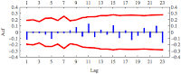
Just for fun, this is the residual autocorrelation of an AR(5) regressed with the crime series data from above:

Not a model anyone should ever depend on. The files used in this post can be found here.