Recently, CNN did a report on the high number of homicides that is plaguing Chicago. One of the sure fire solutions suggested was to place more police in the areas where these killings occur. It got me wondering where these homicides actually occur.
Using the code from my previous post, I called the crime API that the city of Chicago provides and plotted out all the reported homicides between August 1st, 2011 and May 31st, 2012. There were 403 in total.
Now where did these incidents occur?
Initially it looks as if the homicides are wide spread throughout the city. However, if we do a breakdown by neighborhood it becomes obvious that some are much worse off than others. Below is a table of each Chicago neighborhood and its associated number of homicides between August 1st, 2011 and May 31st, 2012. I've also provided a more convenient graphical representation of this table. The Mathematica code and data files I used for this post can be found here.
Showing posts with label mathematica. Show all posts
Tuesday, July 3, 2012
Wednesday, June 27, 2012
Hidden Markov Model of Chicago Crimes
This is a bit of a side note from my attempts to model the number of daily crimes in the city of Chicago. I've been treating the Chicago crime data as a parametric random process where the parameters of the stochastic process can be estimated in a well-defined manner. My first few attempts used various autoregressive models that assumed the crime data was a signal that cross-correlated with itself. From my knowledge of statistics, this is the proper and prescribed treatment for the data. But I have been wondering how well a strictly stochastic model like the Hidden Markov Model (HMM) will perform.
A hidden Markov model is not that hard of a conceptual stretch when applied to crime modeling. Lets assume that all criminal activities in Chicago evolved according to a Markov process, which may have a finite or infinite amount of states. The underlying Markov process is not directly observable because these states are hidden. Luckily, for each state there is an associated stochastic process which produces an observable signal (a crime report). So as this criminal system in Chicago evolves over time, delegated by the hidden Markov chain, it produces crime reports as observable outcomes.
For a full explanation of the mathematical theory behind HMMs please refer to this article by Lawrence Rabiner. Even though Rabiner focuses on HMM applications to speech recognition, it covers in great detail the theory used in my implementation. To simplify things for myself and to cut down on computation time, I created a hidden Markov model with univariate Gaussian outcomes. The model is fitted using a maximum likelihood estimation, where the values of the parameters are those that maximizes the likelihood of the observed data. Here, I used the Baum-Welch Algorithm for estimating the maximum likelihood.
The observed Chicago crime data is the total number of daily reported crimes between July 1, 2011 and March 31, 2012. A log difference transformation of this data was performed to create a more normal distribution of observables. This is all done in Mathematica with six lines of code:
As an example of how to use these functions, lets generate a two state fit with the log differenced crime data. The first step is to generate a random initial parameter set. To hedge the risk of generating a few really bad initial guesses I chose to generate a set of 20 initial guess and run them for 10 iterations. From this set, I then chose the candidate with the highest loglikelihood. This candidate will then be used as a starting point for fitting the model.
To cut down on unnecessary typing, I have written a Do loop to evaluate models with different number of states and used a For loop to create a table of the different models with their associated BIC.
By the BIC, it seems that a HMM with two univariate Gaussian states is the best model. If we examine the Markov chain equilibrium distribution, it seems crimes in Chicago are at a highly volatile with decreasing crimes state about 91% of the time and a low volatility with moderate increases in crimes state about 9% of the time. Looking at the main diagonal of the transition matrix, the large transitions indicate that if crimes in Chicago are found in one state then it will stay in that state for a while.
That is all for now, I'll try to create a simulation with the HMM data for the next post. All the files used for this post can be found here.
A hidden Markov model is not that hard of a conceptual stretch when applied to crime modeling. Lets assume that all criminal activities in Chicago evolved according to a Markov process, which may have a finite or infinite amount of states. The underlying Markov process is not directly observable because these states are hidden. Luckily, for each state there is an associated stochastic process which produces an observable signal (a crime report). So as this criminal system in Chicago evolves over time, delegated by the hidden Markov chain, it produces crime reports as observable outcomes.
For a full explanation of the mathematical theory behind HMMs please refer to this article by Lawrence Rabiner. Even though Rabiner focuses on HMM applications to speech recognition, it covers in great detail the theory used in my implementation. To simplify things for myself and to cut down on computation time, I created a hidden Markov model with univariate Gaussian outcomes. The model is fitted using a maximum likelihood estimation, where the values of the parameters are those that maximizes the likelihood of the observed data. Here, I used the Baum-Welch Algorithm for estimating the maximum likelihood.
The observed Chicago crime data is the total number of daily reported crimes between July 1, 2011 and March 31, 2012. A log difference transformation of this data was performed to create a more normal distribution of observables. This is all done in Mathematica with six lines of code:
csv = Import[
"https://data.cityofchicago.org/api/views/x2n5-8w5q/rows.csv",
"CSV"];
start = "07/01/2011"; end = "03/31/2012";
range = Join[
First[Position[
If[StringMatchQ[#, start ~~ __], 1, 0] & /@
Drop[csv, 1][[All, 2]], 1]] + 1,
Last[Position[
If[StringMatchQ[#, end ~~ __], 1, 0] & /@
Drop[csv, 1][[All, 2]], 1]] + 1];
crimeseries =
Tally[DateString[
DateList[{ToString[#], {"Month", "/", "Day", "/", "Year", " ",
"Hour12", ":", "Minute", " ", "AMPM"}}], {"MonthName", " ",
"Day", " ", "Year"}] & /@ Take[csv, range][[All, 2]]];
The HMM fitting of the crime data uses three functions I created in Mathematica:
MarkovChainEquilibrium[TransitionMatrix_] :=
Inverse[Transpose[TransitionMatrix] -
IdentityMatrix[Length[TransitionMatrix]] + 1].ConstantArray[1,
Length[TransitionMatrix]];
RandomInitial[Data_, States_] := Module[
{TransMat, i, vnGamma, ProbVec, StateMean, vnQ, StateStD, t, mnW},
TransMat = (#/Total[#]) & /@ (RandomReal[{0.01, 0.99}, {States,
States}]);
ProbVec = MarkovChainEquilibrium[TransMat];
StateMean = ((#/Total[#]) &[
RandomReal[{-0.99, 0.99}, States]]) Mean[Data];
StateStD =
Sqrt[((#/Total[#]) &[RandomReal[{0.1, 0.99}, States]]) Variance[
Data]];
{ProbVec, TransMat, StateMean, StateStD}];
Options[HMM] = {"LikelihoodTolerance" -> 10^(-7),
"MaxIterations" -> 500};
HMM[Data_, {InitialIota_, InitialA_, InitialMean_, InitialStD_},
OptionsPattern[]] := Module[
{TransMat, matAlpha, matB, matBeta, nBIC, matGamma, ProbVec,
StateLogLikelihood, iMaxIter, StateMean, iN, StateNu, StateStD, t,
iT, nTol, matWeights, matXi},
nTol = OptionValue["LikelihoodTolerance"];
iMaxIter = OptionValue["MaxIterations"];
iT = Length[Data]; iN = Length[InitialA];
ProbVec = InitialIota; TransMat = InitialA;
StateMean = InitialMean; StateStD = InitialStD;
matB =
Table[PDF[NormalDistribution[StateMean[[#]], StateStD[[#]]],
Data[[t]]] & /@ Range[iN], {t, 1, iT}];
matAlpha = Array[0. &, {iT, iN}];
StateNu = Array[0. &, iT];
matAlpha[[1]] = ProbVec matB[[1]];
StateNu[[1]] = 1/Total[matAlpha[[1]]];
matAlpha[[1]] *= StateNu[[1]];
For[t = 2, t <= iT, t++,
matAlpha[[t]] = (matAlpha[[t - 1]].TransMat) matB[[t]];
StateNu[[t]] = 1/Total[matAlpha[[t]]];
matAlpha[[t]] *= StateNu[[t]]];
StateLogLikelihood = {-Total[Log[StateNu]]};
Do[matBeta = Array[0. &, {iT, iN}];
matBeta[[iT, ;;]] = StateNu[[iT]];
For[t = iT - 1, t >= 1, t--,
matBeta[[t]] =
TransMat.(matBeta[[t + 1]] matB[[t + 1]]) StateNu[[t]]];
matGamma = (#/Total[#]) & /@ (matAlpha matBeta);
matXi = Array[0. &, {iN, iN}];
For[t = 1, t <= iT - 1, t++,
matXi += (#/Total[Flatten[#]]) &[
TransMat KroneckerProduct[matAlpha[[t]],
matBeta[[t + 1]] matB[[t + 1]]]]];
TransMat = (#/Total[#]) & /@ matXi;
ProbVec = matGamma[[1]];
matWeights = (#/Total[#]) & /@ Transpose[matGamma];
StateMean = matWeights.Data;
StateStD = Sqrt[Total /@ (matWeights (Data - # & /@ StateMean)^2)];
matB =
Table[PDF[NormalDistribution[StateMean[[#]], StateStD[[#]]],
Data[[t]]] & /@ Range[iN], {t, 1, iT}];
matAlpha = Array[0. &, {iT, iN}];
StateNu = Array[0. &, iT];
matAlpha[[1]] = ProbVec matB[[1]];
StateNu[[1]] = 1/Total[matAlpha[[1]]];
matAlpha[[1]] *= StateNu[[1]];
For[t = 2, t <= iT, t++,
matAlpha[[t]] = (matAlpha[[t - 1]].TransMat) matB[[t]];
StateNu[[t]] = 1/Total[matAlpha[[t]]];
matAlpha[[t]] *= StateNu[[t]]];
StateLogLikelihood =
Append[StateLogLikelihood, -Total[Log[StateNu]]];
If[StateLogLikelihood[[-1]]/StateLogLikelihood[[-2]] - 1 <= nTol,
Break[]],
{iMaxIter}];
nBIC = -2 StateLogLikelihood[[-1]] + (iN (iN + 2) - 1) Log[iT];
{"\[Iota]" -> ProbVec, "a" -> TransMat, "\[Mu]" -> StateMean,
"\[Sigma]" -> StateStD, "\[Gamma]" -> matGamma, "BIC" -> nBIC,
"LL" -> StateLogLikelihood}];
The first function computes the equilibrium distribution for an ergodic Markov chain. The second function generates a random parameter set with inputs of the observed data and the number of states. Output from the second function is a list containing the initial state probability vector, the transition matrix of the Markov chain, the mean of each state, and the standard deviation of each state. The third function is the maximum likelihood estimated fit of the HMM. It takes inputs of the observed data and a random parameter set from the second function. The output from the third function is a list that contains the initial state probability vector, the transition matrix, the mean vector, the standard deviation vector, a vector of periodic state probabilities, the Bayesian Information Criterion (BIC) for the fit, and a history of the loglikelihood for each iteration.As an example of how to use these functions, lets generate a two state fit with the log differenced crime data. The first step is to generate a random initial parameter set. To hedge the risk of generating a few really bad initial guesses I chose to generate a set of 20 initial guess and run them for 10 iterations. From this set, I then chose the candidate with the highest loglikelihood. This candidate will then be used as a starting point for fitting the model.
guess = HMM[crimedifference[[All, 2]], #, "MaxIterations" -> 10] & /@
Table[RandomInitial[crimedifference[[All, 2]], 2], {20}];
bestguessLL =
Flatten[Position[#, Max[#]] &[Last["LL" /. #] & /@ guess]][[1]];
hmmfit = HMM[
crimedifference[[All,
2]], {"\[Iota]", "a", "\[Mu]",
"\[Sigma]"} /. (guess[[bestguessLL]])];
It is usually a good idea to check the convergence of the likelihood function to make sure nothing has gone awry.
ListPlot["LL" /. hmmfit, PlotRange -> All]
To cut down on unnecessary typing, I have written a Do loop to evaluate models with different number of states and used a For loop to create a table of the different models with their associated BIC.
MaxGaussians = 3;
Do[InitialGuess["Crimes", i] =
HMM[crimedifference[[All, 2]], #, "MaxIterations" -> 10] & /@
Table[RandomInitial[crimedifference[[All, 2]], i], {20}];
BestGuessLL["Crimes", i] =
Flatten[Position[#, Max[#]] &[
Last["LL" /. #] & /@ InitialGuess["Crimes", i]]][[1]];
FittedHMM["Crimes", i] =
HMM[crimedifference[[All,
2]], {"\[Iota]", "a", "\[Mu]",
"\[Sigma]"} /. (InitialGuess["Crimes", i][[
BestGuessLL["Crimes", i]]])],
{i, 1, MaxGaussians, 1}]
bic = {}; states = {};
For[i = 1, i < MaxGaussians + 1, i++, AppendTo[states, i];
j = "BIC" /. FittedHMM["Crimes", i]; AppendTo[bic, j]]
TableForm[Transpose[{states, bic}],
TableHeadings -> {None, {"#States", "BIC"}},
TableAlignments -> Center]
By the BIC, it seems that a HMM with two univariate Gaussian states is the best model. If we examine the Markov chain equilibrium distribution, it seems crimes in Chicago are at a highly volatile with decreasing crimes state about 91% of the time and a low volatility with moderate increases in crimes state about 9% of the time. Looking at the main diagonal of the transition matrix, the large transitions indicate that if crimes in Chicago are found in one state then it will stay in that state for a while.
Print["Equilibrium Distribution = ", MatrixForm[MarkovChainEquilibrium["a" /. FittedHMM["Crimes", 2]]]] Print["Transition Matrix from Data = ", MatrixForm["a" /. FittedHMM["Crimes", 2]]]
That is all for now, I'll try to create a simulation with the HMM data for the next post. All the files used for this post can be found here.
Tuesday, June 26, 2012
First Attempt at Modeling Crime in Chicago, Part 3
I've been trying to keep my attempts to model crimes in Chicago relatively simple. I was hoping to be able to generate some decent predictions by examining a few months of crime data as a signal using a simple autoregressive moving average model (ARMA). And I've finally made some progress!
I found that a ARMA(2, 3) process acts as a reasonable descriptor for the first difference of the crime data between July 1st, 2011 and March 31st, 2012. The graphs above are simulations for April 2012 that were generated with my regressed ARMA(2, 3) parameters. My choices of using an ARMA model and fitting the first difference of the data is explained in a previous post. The Mathematica code that performs the fitting and diagnostic checks is quite extensive so I may release the work for this post as a package in a later post and document all of the functions then. But if you want to play around with my code and do not mind working with Mathematica, you can find everything used to create this post here (Warning! It is still a work in progress).
Thursday, June 21, 2012
Simple Step to Create a Slicker Site
In my last few posts I had been skimping on a great deal of procedural details and presented only on some fun results. This could be blamed on my dwindling resources of free time and my compulsion to make things presentable. These reasons are significant hurdles to blogging about a semi-programming language like Mathematica, a document markup language like LaTeX, or intermediate-level languages like C++. Other than displaying these codes as plaintext or a cropped screenshot, there are few efficient options to posting them and even fewer to display the code's syntax in a manner that would fit a personalized blog design on Blogger.
A fantastic solution to this problem is the combined use of google-code-prettify and SyntaxHighlighter. The setup of these JavaScripts on Blogger is quite simple, the configurations are limitless, and the results are visually appealing.
For example, if I wanted to write a quick crazy mathematica post on how to gather all the historical drawings for the Mega Millions lottery. It would've taken me some time to create a Blogger-ready-sized png picture of the code to upload to Blogger and it would've annoyed my blog readers because they would have to manually type out the code below.
Using google-code-prettify I can copy and paste my code in nanoseconds and my readers would also be able to use the code to pick their winning Mega Millions numbers right away.
<link href='INSERT LINK TO prettify.css' rel='stylesheet' type='text/css'/>
<script language='javascript' src='INSERT LINK TO prettify.js' type='text/javascript'/>
<script language='javascript' src='INSERT LINK TO lang-mma.js' type='text/javascript'/>
<script type='text/javascript'>
document.addEventListener('DOMContentLoaded',function() {
prettyPrint();
});
</script>
You can now use the script to create Mathematica styled syntax in a Blogger post by using the tag name "pre" and the "prettyprint" class in the HTML code of a Blogger post. Try it out with the Mega Millions Mathematica code from above.
<pre class="prettyprint lang-mma">
<!--Paste Mathematica code here-->
</pre>
As seen on his post for other languages, I prefer to use SyntaxHighlighter over google-code-prettify. The instructions on how to setup and use SyntaxHighlighter on Blogger can be found here, so I will not be covering it - unless requested. You can find all the files used for this post here. Happy Blogging Everyone!
A fantastic solution to this problem is the combined use of google-code-prettify and SyntaxHighlighter. The setup of these JavaScripts on Blogger is quite simple, the configurations are limitless, and the results are visually appealing.
For example, if I wanted to write a quick crazy mathematica post on how to gather all the historical drawings for the Mega Millions lottery. It would've taken me some time to create a Blogger-ready-sized png picture of the code to upload to Blogger and it would've annoyed my blog readers because they would have to manually type out the code below.
Using google-code-prettify I can copy and paste my code in nanoseconds and my readers would also be able to use the code to pick their winning Mega Millions numbers right away.
dat[x_] :=
Drop[Drop[
Flatten[Import[
"http://www.usamega.com/mega-millions-history.asp?p=" <>
ToString[x] <> "", "Data"], 4], 5], -3]
n = 61;
dat1 = ToString[Flatten[dat[#] & /@ Range[n], 1]];
data = ToExpression[
StringReplace[dat1, {"\[CenterDot]" -> ",", "+" -> ","}]];
number1 = data[[All, 4]];
number2 = data[[All, 5]];
number3 = data[[All, 6]];
number4 = data[[All, 7]];
number5 = data[[All, 8]];
megaball = data[[All, 9]];
To get google-code-prettify set up on Blogger, you will need a free DropBox or box account and the three files I provide here. The lang-mma.js and prettify.css files I have provided for this post were forked from the Mathematica - Stack Exchange. Then follow these steps:- Place the uncompressed files anywhere in your preferred cloud drive account.
- Get the sharable hyperlinks of those three files.
- In Blogger (with the new 2012 interface) go to the Template tab on the left, then navigate to the Edit HTML button and proceed.
- Copy and paste the following code into your HTML template (best spot would be right before </head>) and insert the appropriate links in step 2 and save.
You can now use the script to create Mathematica styled syntax in a Blogger post by using the tag name "pre" and the "prettyprint" class in the HTML code of a Blogger post. Try it out with the Mega Millions Mathematica code from above.
As seen on his post for other languages, I prefer to use SyntaxHighlighter over google-code-prettify. The instructions on how to setup and use SyntaxHighlighter on Blogger can be found here, so I will not be covering it - unless requested. You can find all the files used for this post here. Happy Blogging Everyone!
Tuesday, June 12, 2012
First Attempt at Modeling Crime in Chicago, Part 2
In the last post, my main goal was to develop a Mathematica 8 program that could regress coefficients for general autoregressive (AR) models. In my excitement, I skipped an essential step of data modeling. I forgot to check if the data could be accurately described by an AR model.
To keep things simple for the remainder of my attempts to model the number of daily crimes in Chicago, I will be using only the data between July 1st, 2011 and March 31st, 2012. This will also give me a reason to use the new Data section of my blog.
\[G_{k}=\frac{V(z_{t+k}-z_{t})}{V(z_{t+1}-z_{t})},\;k=1,2,3...\]
\[d^{k}_{t}=z_{t+k}-z_{t}\]
In Mathematica, a sample variogram can be calculated accordingly:
LagDifferences[list_, k_Integer?Positive] /; k < Length[list] := Drop[list, k] - Drop[list, -k];
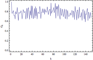
Now we can finally move on to model selection. As a rule of thumb, an AR(p) model can adequately model a set of data if the autocorrelation function (Acf) plot looks like an infinitely damped exponential or sine wave that tails off and the partial autocorrelation function (PAcf) plot is cut off after p lags. Plots of the variogram, autocorrelation function, and partial autocorrelation function for the Chicago crime data and differences of the data are shown below.
It looks like taking the first difference will produce a more stationary time series. The large negative autocorrelation at lag 1 in both the Acf and PAcf plot suggests the data may be better described with a moving average model component rather than with just an autoregressive model. Looks like it is bullocks on me for jumping the gun. I'll be back next post with a moving average model made in Mathematica. Until then, have fun with the source files for this post here.
To keep things simple for the remainder of my attempts to model the number of daily crimes in Chicago, I will be using only the data between July 1st, 2011 and March 31st, 2012. This will also give me a reason to use the new Data section of my blog.
Before examining the legitimacy of an AR model selection, I need to check if the data is stationary. The basis for any time series analysis is a stationary time series, because essentially we can only develop models and forecasts for stationary time series. In my experience, I have found no clear demarcation between stationary and non-stationary data. The usual approach to determine stationarity is to plot the autocorrelation function and if the plot doesn't dampen at long lags than the data is most likely not stationary. This logic escapes me. It may be because my statistical skills come from my engineering and computational chemistry training but I don't think the autocorrelation function is defined for non-stationary processes.
One of the tricks to transform a non-stationary dataset to a stationary one is to take the difference of the non-stationary dataset. So for me, a variogram is the more logical tool for determining stationarity. A variogram gives a ratio of the variance of differences some k time units apart and the variance of the differences only one time unit apart. If you look at the equations below, as k goes to infinity the difference between k lag and k+1 lag will eventually be the same. Ideally, you can conclude a dataset is stationary when the variogram shows a stable asymptote.
\[G_{k}=\frac{V(z_{t+k}-z_{t})}{V(z_{t+1}-z_{t})},\;k=1,2,3...\]
where
\[V(z_{t+k}-z_{t})=\frac{\sum_{t=1}^{n-k}(d^{ k}_{t}-(n-k)^{-1}\sum d^{ k}_{t})^2}{n-k-1}\]\[d^{k}_{t}=z_{t+k}-z_{t}\]
In Mathematica, a sample variogram can be calculated accordingly:
LagDifferences[list_, k_Integer?Positive] /; k < Length[list] := Drop[list, k] - Drop[list, -k];
Variogram[list_, k_] := (#/First@#) &@(Variance /@ Table[LagDifferences[list, i], {i, k}]);
Now we can finally move on to model selection. As a rule of thumb, an AR(p) model can adequately model a set of data if the autocorrelation function (Acf) plot looks like an infinitely damped exponential or sine wave that tails off and the partial autocorrelation function (PAcf) plot is cut off after p lags. Plots of the variogram, autocorrelation function, and partial autocorrelation function for the Chicago crime data and differences of the data are shown below.
| Variogram | |
|---|---|
| Crime Series |
|
| 1st Difference |
|
| 2nd Difference |
|
| Autocorrelation | Partial Autocorrelation | |
|---|---|---|
| Crime Series |
|
|
| 1st Difference |
|
|
| 2nd Difference |
|
|
It looks like taking the first difference will produce a more stationary time series. The large negative autocorrelation at lag 1 in both the Acf and PAcf plot suggests the data may be better described with a moving average model component rather than with just an autoregressive model. Looks like it is bullocks on me for jumping the gun. I'll be back next post with a moving average model made in Mathematica. Until then, have fun with the source files for this post here.
Tuesday, June 5, 2012
First Attempt at Modeling Crime in Chicago
In my last post, I showed how to use the Socrata Open Data API (SODA) to download the data of the crimes reported in Chicago, how to plot the locations, and how to count the number of crimes that occurred in a certain area. This post will chronicle my first attempts to model that data in Mathematica.
The time series analysis add-on to Mathematica 8 costs about $295. So I've decided to write my own autoregressive model (AR) package as a start to modeling the crimes in Chicago. My AR code in Mathematica is based off the FitAR R-package and its associated paper. The mathematics and derivations of autoregressive models are already heavily covered on other websites, so I will not be explaining it here. The alpha version of my code can be found here, note it is not complete and does not yet have all the functions of FitAR or the Mathematica time series add-on.
My code, at this point, does provide fits that are comparable to the FitAR package. Using the default "lynx" data in R the following fits and associated residual autocorrelation plots were produced:
Now that I know my code is correct, the next step will be figuring out if an autoregressive model can properly describe the crime data from Chicago. The lynx data from above is almost trivial when compared to the chaotic mess of crime data.
Just for fun, this is the residual autocorrelation of an AR(5) regressed with the crime series data from above:
Not a model anyone should ever depend on. The files used in this post can be found here.
The time series analysis add-on to Mathematica 8 costs about $295. So I've decided to write my own autoregressive model (AR) package as a start to modeling the crimes in Chicago. My AR code in Mathematica is based off the FitAR R-package and its associated paper. The mathematics and derivations of autoregressive models are already heavily covered on other websites, so I will not be explaining it here. The alpha version of my code can be found here, note it is not complete and does not yet have all the functions of FitAR or the Mathematica time series add-on.
My code, at this point, does provide fits that are comparable to the FitAR package. Using the default "lynx" data in R the following fits and associated residual autocorrelation plots were produced:
Mathematica
| MLE | sd | Z-ratio | |
|---|---|---|---|
| phi(1) | 0.71729 | 0.0652589 | 10.9914 |
| mu | 1537.94 | 364.477 | 4.21957 |
| MLE | sd | Z-ratio | |
|---|---|---|---|
| phi(1) | 1.12428 | 0.0905874 | 12.411 |
| phi(2) | -0.716667 | 0.136707 | -5.24237 |
| phi(3) | 0.262661 | 0.136707 | 1.92135 |
| phi(4) | -0.253983 | 0.0905874 | -2.80374 |
| mu | 1537.94 | 135.755 | 11.3288 |
| MLE | sd | Z-ratio | |
|---|---|---|---|
| phi(1) | 0.820455 | 0.0178649 | 45.9256 |
| phi(2) | -0.632818 | 0.0972914 | -6.50436 |
| phi(4) | -0.141951 | 0.0684639 | -2.07337 |
| phi(5) | 0.141893 | 0.0748193 | 1.89647 |
| phi(7) | 0.202038 | 0.0992876 | 2.03488 |
| phi(10) | -0.314105 | 0.0917768 | -3.42249 |
| phi(11) | -0.368658 | 0.0870617 | -4.23444 |
| mu | 6.68591 | 0.100657 | 66.4225 |
R
| MLE | sd | Z-ratio | |
|---|---|---|---|
| phi(1) | 0.717303 | 0.0652577 | 10.9918 |
| mu | 1538.02 | 363.986 | 4.22548 |
| MLE | sd | Z-ratio | |
|---|---|---|---|
| phi(1) | 1.12463 | 0.0905803 | 12.4158 |
| phi(2) | -0.717396 | 0.1367150 | -5.24738 |
| phi(3) | 0.263355 | 0.136715 | 1.92630 |
| phi(4) | -0.254273 | 0.0905803 | -2.80716 |
| mu | 1538.02 | 135.469 | 11.3533 |
| MLE | sd | Z-ratio | |
|---|---|---|---|
| phi(1) | 0.8204490 | 0.01786005 | 45.937651 |
| phi(2) | -0.6328433 | 0.09731087 | -6.503316 |
| phi(4) | -0.1420888 | 0.06847123 | -2.075161 |
| phi(5) | 0.1421388 | 0.07481409 | 1.899894 |
| phi(7) | 0.2021250 | 0.09927376 | 2.036036 |
| phi(10) | -0.3140954 | 0.09178210 | -3.422186 |
| phi(11) | -0.3686589 | 0.08706171 | -4.234455 |
| mu | 6.6859329 | 0.09999207 | 66.864631 |
Now that I know my code is correct, the next step will be figuring out if an autoregressive model can properly describe the crime data from Chicago. The lynx data from above is almost trivial when compared to the chaotic mess of crime data.
![]() |
| Time Series Plot of lynx data |
![]() |
| Plot of daily totals of crimes in Chicago. |
Just for fun, this is the residual autocorrelation of an AR(5) regressed with the crime series data from above:
Not a model anyone should ever depend on. The files used in this post can be found here.
Monday, May 7, 2012
Chicago Crime - Updated
I was a bit dismayed to discover that the EveryBlock API stopped working. One of my most popular posts, Chicago Crime, depended on this API heavily.
Here I present an alternative data source for my previous post and a fun update. The update is a quick and dirty method to create popular crime density plots, as shown below.
In the spirit of transparency, the city of Chicago has taken the initiative to electronically release a great deal of data with Socrata Open Data API (SODA). Luckily for us, this release includes all filed police reports. The records available through this API range from the year 2001 to the present, which dwarfs the two week range provided by EveryBlock's API. However, I would not recommend downloading all of this data as the text file is approximately 2GB in size.
In this post I use only the filed police reports from one year prior to present. The data is available in both JSON and CSV format. I only use the CSV format here for the convenience of those with an earlier version of Mathematica. To import this data into Mathematica:
A plot of all reported crimes in Chicago between February 1st and March 31st of 2012 was created with the data.
Plot of incidents for any period within the year can be easily created with the following Mathematica code. Restrict the data to the range of interest by replacing the dates of the start and end strings. Dates must be in the format of mm/dd/yyyy. This code simply finds the positions of the strings that match the inputed dates and plots the daily totals of incidents.
The data can be parsed into primary descriptions including arson, homicide, sex offense, weapons violation, crim sexual assault, interfere with public officer, gambling, public peace violation, criminal trespass, liquor law violation, assault, deceptive practice, burglary, criminal damage, robbery, motor vehicle theft, offense involving children, narcotics, theft, other offense, and battery. Below is the plot and code to filter for only narcotics incidents.
A secondary description can also be used to parse the data. Some secondary descriptions include aggravated: handgun, poss: crack, armed: handgun, harassment by telephone, poss: heroin(white), to land, retail theft, unlawful entry, strongarm - no weapon, to property, poss: cannabis 30gms or less, from building, $500 and under, forcible entry, to vehicle, domestic battery simple, simple, automobile, over $500, telephone threat, and wireroom/sports. Below is the plot and code to filter for incidents with a primary description of narcotics and a secondary description of poss: cannabis 30gms or less.
The incidents may also be separated into ones where arrests were made and ones where no arrests were made. Below is code to filter for incidents with a primary description of narcotics and a secondary description of poss: cannabis 30gms or less with arrests and without. Both plots comparing to total narcotics incidents are shown.
The method to display where certain incidents occur in chicago is similar to my previous post, Chicago Crime. Please refer to that posting for a more detailed explanation on how to create the plot below. The plot here is a geographical visualization of where arrests occurred relating to incidents of narcotics with possession of cannabis with 30 grams or less.
The method to tabulate the number of incidents within neighborhoods is also similar to my previous post, Chicago Crime. This calculation totals the numbers of incidents within each neighborhood boundary. It is the most costly in computational time and power because of the generality in the counting code that allows it to use any boundaries (such as census tracts, police beats, etc.) The tabulation of arrests made relating to incidents of narcotics with possession of cannabis with 30 grams or less in each neighborhood is presented.
While doing some initial research for this post, I found "crime hotspots" as a popular visualization option. A similar visualization is easily created in mathematica with three simple lines of code.
The Mathematica code used in this post can be downloaded here. Some fun analysis of crimes in chicago will follow in future posts.
Here I present an alternative data source for my previous post and a fun update. The update is a quick and dirty method to create popular crime density plots, as shown below.
In this post I use only the filed police reports from one year prior to present. The data is available in both JSON and CSV format. I only use the CSV format here for the convenience of those with an earlier version of Mathematica. To import this data into Mathematica:
A plot of all reported crimes in Chicago between February 1st and March 31st of 2012 was created with the data.
Plot of incidents for any period within the year can be easily created with the following Mathematica code. Restrict the data to the range of interest by replacing the dates of the start and end strings. Dates must be in the format of mm/dd/yyyy. This code simply finds the positions of the strings that match the inputed dates and plots the daily totals of incidents.
The data can be parsed into primary descriptions including arson, homicide, sex offense, weapons violation, crim sexual assault, interfere with public officer, gambling, public peace violation, criminal trespass, liquor law violation, assault, deceptive practice, burglary, criminal damage, robbery, motor vehicle theft, offense involving children, narcotics, theft, other offense, and battery. Below is the plot and code to filter for only narcotics incidents.
A secondary description can also be used to parse the data. Some secondary descriptions include aggravated: handgun, poss: crack, armed: handgun, harassment by telephone, poss: heroin(white), to land, retail theft, unlawful entry, strongarm - no weapon, to property, poss: cannabis 30gms or less, from building, $500 and under, forcible entry, to vehicle, domestic battery simple, simple, automobile, over $500, telephone threat, and wireroom/sports. Below is the plot and code to filter for incidents with a primary description of narcotics and a secondary description of poss: cannabis 30gms or less.
The incidents may also be separated into ones where arrests were made and ones where no arrests were made. Below is code to filter for incidents with a primary description of narcotics and a secondary description of poss: cannabis 30gms or less with arrests and without. Both plots comparing to total narcotics incidents are shown.
The method to display where certain incidents occur in chicago is similar to my previous post, Chicago Crime. Please refer to that posting for a more detailed explanation on how to create the plot below. The plot here is a geographical visualization of where arrests occurred relating to incidents of narcotics with possession of cannabis with 30 grams or less.
The method to tabulate the number of incidents within neighborhoods is also similar to my previous post, Chicago Crime. This calculation totals the numbers of incidents within each neighborhood boundary. It is the most costly in computational time and power because of the generality in the counting code that allows it to use any boundaries (such as census tracts, police beats, etc.) The tabulation of arrests made relating to incidents of narcotics with possession of cannabis with 30 grams or less in each neighborhood is presented.
While doing some initial research for this post, I found "crime hotspots" as a popular visualization option. A similar visualization is easily created in mathematica with three simple lines of code.
The Mathematica code used in this post can be downloaded here. Some fun analysis of crimes in chicago will follow in future posts.
Thursday, April 19, 2012
Can I Trust Wikipedia?
A question as dreaded as "Who's on first?" And one that I am forced to ask as I feel lucky often. One quick and fun way to address how much you can trust a wikipedia article is by looking at what else a contributor edits. This can easily be done through the magic of the MediaWiki API and Mathematica. Here is the result, with a CNN inspired example, of Mitt Romney's wikipedia article from April 19th, 2012.
Personally, I see red flags when contributors of the Mitt Romney article are also subject-matter experts of Katy Perry, Springfield (The Simpsons), and Savage Love. I wouldn't put too much faith in its accuracy.
A copy of the notebook can be downloaded here. To use it, simply copy the title of the wikipedia article of interest and paste it into the third line. More to come the next time I skip lunch!
![]() |
| The top 20 contributors to the Mitt Romney wikipedia article are highlighted in yellow and common articles edited by these contributors are highlighted in blue. |
Personally, I see red flags when contributors of the Mitt Romney article are also subject-matter experts of Katy Perry, Springfield (The Simpsons), and Savage Love. I wouldn't put too much faith in its accuracy.
A copy of the notebook can be downloaded here. To use it, simply copy the title of the wikipedia article of interest and paste it into the third line. More to come the next time I skip lunch!
Saturday, November 26, 2011
Making Sense of Census-less Data
I have always found that supplemental 3D visualizations help provide better insights on census data. While playing with the compiled data from the 2000 census, from cityofchicago.org, I found an interesting anomaly.
After some investigation, I found the red spike represents 15 families with a median income of $255,000. Was there mischief afoot by those 15 families?
I'll let the more curious readers decide. Attached here is the census data and a Mathematica notebook. The notebook has been generalized to allow users to create 3D visualizations of all provided census data.
Download here
Thursday, November 10, 2011
Batman Letterhead
After reading a post from HardOCP that gave the roots of the Batman symbol, I could not help imagining the letterhead of the world's greatest detective. The letterhead needs to say "Batman is classy."
I created this letterhead using the "Batman equation", Mathematica, and LaTeX. The computer in the Bat Cave is probably Unix-based and cannot use Microsoft Word. Therefore, Batman must use LaTeX. The first step to creating this letterhead is to plot the symbol. A post from Playing With Mathematica has done this for me already with seven simple lines.
To extract the points used for the final plot the following command must be executed for each root equation.
After extracting and compiling all data points into one .dat file, we are ready to create the letterhead in LaTeX. The following LaTeX code relies on the pstricks and pst-plot packages. It plots the points in the saved data file and creates the bar that separates Batman's contact information.
\begin{document}
\readdata{\BatData}{BatData.dat}
\noindent\begin{minipage}[b]{5cm}
\begin{center}
\psset{xunit=0.35cm,yunit=0.5cm}
\begin{pspicture}(0,0)(0,2)
\listplot[plotstyle=dots]{\BatData}
\end{pspicture}
\end{center}
\end{minipage}
\hfill
\begin{minipage}[b]{7cm}
\begin{flushright}
\footnotesize{\itshape 1007 Mountain Drive {\scriptsize$\bullet$} Gotham City, NY 10027}
\end{flushright}
\end{minipage}
\vskip-2mm
{\hspace{40mm}\hfill\rule[0.5mm]{130mm}{0.5pt}}
\vskip-2mm
\hfill
\begin{minipage}[b]{7cm}
\begin{flushright}
\footnotesize{\itshape 555.555.5555 {\scriptsize$\bullet$} \href{mailto:Bruce@WayneCorp.com}{Bruce@WayneCorp.com}}
\end{flushright}
\end{minipage}
I created this letterhead using the "Batman equation", Mathematica, and LaTeX. The computer in the Bat Cave is probably Unix-based and cannot use Microsoft Word. Therefore, Batman must use LaTeX. The first step to creating this letterhead is to plot the symbol. A post from Playing With Mathematica has done this for me already with seven simple lines.
The Show function is used to overlay the six plots to reveal the desired product.
To extract the points used for the final plot the following command must be executed for each root equation.
After extracting and compiling all data points into one .dat file, we are ready to create the letterhead in LaTeX. The following LaTeX code relies on the pstricks and pst-plot packages. It plots the points in the saved data file and creates the bar that separates Batman's contact information.
\begin{document}
\readdata{\BatData}{BatData.dat}
\noindent\begin{minipage}[b]{5cm}
\begin{center}
\psset{xunit=0.35cm,yunit=0.5cm}
\begin{pspicture}(0,0)(0,2)
\listplot[plotstyle=dots]{\BatData}
\end{pspicture}
\end{center}
\end{minipage}
\hfill
\begin{minipage}[b]{7cm}
\begin{flushright}
\footnotesize{\itshape 1007 Mountain Drive {\scriptsize$\bullet$} Gotham City, NY 10027}
\end{flushright}
\end{minipage}
\vskip-2mm
{\hspace{40mm}\hfill\rule[0.5mm]{130mm}{0.5pt}}
\vskip-2mm
\hfill
\begin{minipage}[b]{7cm}
\begin{flushright}
\footnotesize{\itshape 555.555.5555 {\scriptsize$\bullet$} \href{mailto:Bruce@WayneCorp.com}{Bruce@WayneCorp.com}}
\end{flushright}
\end{minipage}
All of the files discussed in this post can be downloaded here, along with a letter Batman would've sent to The Joker.
Subscribe to:
Posts (Atom)