Showing posts with label Autoregressive modeling. Show all posts

Tuesday, June 26, 2012

First Attempt at Modeling Crime in Chicago, Part 3

I've been trying to keep my attempts to model crimes in Chicago relatively simple. I was hoping to be able to generate some decent predictions by examining a few months of crime data as a signal using a simple autoregressive moving average model (ARMA). And I've finally made some progress!


I found that a ARMA(2, 3) process acts as a reasonable descriptor for the first difference of the crime data between July 1st, 2011 and March 31st, 2012. The graphs above are simulations for April 2012 that were generated with my regressed ARMA(2, 3) parameters. My choices of using an ARMA model and fitting the first difference of the data is explained in a previous post. The Mathematica code that performs the fitting and diagnostic checks is quite extensive so I may release the work for this post as a package in a later post and document all of the functions then. But if you want to play around with my code and do not mind working with Mathematica, you can find everything used to create this post here (Warning! It is still a work in progress).

Tuesday, June 12, 2012

First Attempt at Modeling Crime in Chicago, Part 2

In the last post, my main goal was to develop a Mathematica 8 program that could regress coefficients for general autoregressive (AR) models. In my excitement, I skipped an essential step of data modeling. I forgot to check if the data could be accurately described by an AR model.

To keep things simple for the remainder of my attempts to model the number of daily crimes in Chicago, I will be using only the data between July 1st, 2011 and March 31st, 2012. This will also give me a reason to use the new Data section of my blog.


Before examining the legitimacy of an AR model selection, I need to check if the data is stationary. The basis for any time series analysis is a stationary time series, because essentially we can only develop models and forecasts for stationary time series. In my experience, I have found no clear demarcation between stationary and non-stationary data. The usual approach to determine stationarity is to plot the autocorrelation function and if the plot doesn't dampen at long lags than the data is most likely not stationary. This logic escapes me. It may be because my statistical skills come from my engineering and computational chemistry training but I don't think the autocorrelation function is defined for non-stationary processes.

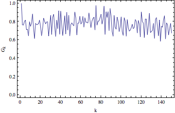
One of the tricks to transform a non-stationary dataset to a stationary one is to take the difference of the non-stationary dataset. So for me, a variogram is the more logical tool for determining stationarity. A variogram gives a ratio of the variance of differences some k time units apart and the variance of the differences only one time unit apart. If you look at the equations below, as k goes to infinity the difference between k lag and k+1 lag will eventually be the same. Ideally, you can conclude a dataset is stationary when the variogram shows a stable asymptote.

\[G_{k}=\frac{V(z_{t+k}-z_{t})}{V(z_{t+1}-z_{t})},\;k=1,2,3...\]
where
\[V(z_{t+k}-z_{t})=\frac{\sum_{t=1}^{n-k}(d^{ k}_{t}-(n-k)^{-1}\sum d^{ k}_{t})^2}{n-k-1}\]
\[d^{k}_{t}=z_{t+k}-z_{t}\]

In Mathematica, a sample variogram can be calculated accordingly:

LagDifferences[list_, k_Integer?Positive] /; k < Length[list] := Drop[list, k] - Drop[list, -k];

Variogram[list_, k_] := (#/First@#) &@(Variance /@ Table[LagDifferences[list, i], {i, k}]);

Now we can finally move on to model selection. As a rule of thumb, an AR(p) model can adequately model a set of data if the autocorrelation function (Acf) plot looks like an infinitely damped exponential or sine wave that tails off and the partial autocorrelation function (PAcf) plot is cut off after p lags. Plots of the variogram, autocorrelation function, and partial autocorrelation function for the Chicago crime data and differences of the data are shown below.

Variogram
Crime Series

1st Difference

2nd Difference


Autocorrelation Partial Autocorrelation
Crime Series


1st Difference


2nd Difference


It looks like taking the first difference will produce a more stationary time series. The large negative autocorrelation at lag 1 in both the Acf and PAcf plot suggests the data may be better described with a moving average model component rather than with just an autoregressive model. Looks like it is bullocks on me for jumping the gun. I'll be back next post with a moving average model made in Mathematica. Until then, have fun with the source files for this post here.

Tuesday, June 5, 2012

First Attempt at Modeling Crime in Chicago

In my last post, I showed how to use the Socrata Open Data API (SODA) to download the data of the crimes reported in Chicago, how to plot the locations, and how to count the number of crimes that occurred in a certain area. This post will chronicle my first attempts to model that data in Mathematica.

The time series analysis add-on to Mathematica 8 costs about $295. So I've decided to write my own autoregressive model (AR) package as a start to modeling the crimes in Chicago. My AR code in Mathematica is based off the FitAR R-package and its associated paper. The mathematics and derivations of autoregressive models are already heavily covered on other websites, so I will not be explaining it here. The alpha version of my code can be found here, note it is not complete and does not yet have all the functions of FitAR or the Mathematica time series add-on.

My code, at this point, does provide fits that are comparable to the FitAR package. Using the default "lynx" data in R the following fits and associated residual autocorrelation plots were produced:


Mathematica

AR(1) Fit
MLEsdZ-ratio
phi(1)0.717290.065258910.9914
mu1537.94364.4774.21957


AR(4) Fit
MLEsdZ-ratio
phi(1)1.124280.090587412.411
phi(2)-0.7166670.136707-5.24237
phi(3)0.2626610.1367071.92135
phi(4)-0.2539830.0905874-2.80374
mu1537.94135.75511.3288


Subset AR(1,2,4,5,7,10,11) Fit
MLEsdZ-ratio
phi(1)0.8204550.017864945.9256
phi(2)-0.6328180.0972914-6.50436
phi(4)-0.1419510.0684639-2.07337
phi(5)0.1418930.07481931.89647
phi(7)0.2020380.09928762.03488
phi(10)-0.3141050.0917768-3.42249
phi(11)-0.3686580.0870617-4.23444
mu6.685910.10065766.4225

R

AR(1) Fit
MLEsdZ-ratio
phi(1)0.7173030.065257710.9918
mu1538.02363.9864.22548


AR(4) Fit
MLEsdZ-ratio
phi(1)1.124630.090580312.4158
phi(2)-0.7173960.1367150-5.24738
phi(3)0.2633550.1367151.92630
phi(4)-0.2542730.0905803-2.80716
mu1538.02135.46911.3533


Subset AR(1,2,4,5,7,10,11) Fit
MLEsdZ-ratio
phi(1)0.82044900.0178600545.937651
phi(2)-0.63284330.09731087-6.503316
phi(4)-0.14208880.06847123-2.075161
phi(5)0.14213880.074814091.899894
phi(7)0.20212500.099273762.036036
phi(10)-0.31409540.09178210-3.422186
phi(11)-0.36865890.08706171-4.234455
mu6.68593290.0999920766.864631


Now that I know my code is correct, the next step will be figuring out if an autoregressive model can properly describe the crime data from Chicago. The lynx data from above is almost trivial when compared to the chaotic mess of crime data.

Time Series Plot of lynx data

Plot of daily totals of crimes in Chicago.

Just for fun, this is the residual autocorrelation of an AR(5) regressed with the crime series data from above:


Not a model anyone should ever depend on. The files used in this post can be found here.