First Attempt at Modeling Crime in Chicago, Part 2

In the last post, my main goal was to develop a Mathematica 8 program that could regress coefficients for general autoregressive (AR) models. In my excitement, I skipped an essential step of data modeling. I forgot to check if the data could be accurately described by an AR model.

To keep things simple for the remainder of my attempts to model the number of daily crimes in Chicago, I will be using only the data between July 1st, 2011 and March 31st, 2012. This will also give me a reason to use the new Data section of my blog.

Before examining the legitimacy of an AR model selection, I need to check if the data is stationary. The basis for any time series analysis is a stationary time series, because essentially we can only develop models and forecasts for stationary time series. In my experience, I have found no clear demarcation between stationary and non-stationary data. The usual approach to determine stationarity is to plot the autocorrelation function and if the plot doesn't dampen at long lags than the data is most likely not stationary. This logic escapes me. It may be because my statistical skills come from my engineering and computational chemistry training but I don't think the autocorrelation function is defined for non-stationary processes.

One of the tricks to transform a non-stationary dataset to a stationary one is to take the difference of the non-stationary dataset. So for me, a variogram is the more logical tool for determining stationarity. A variogram gives a ratio of the variance of differences some k time units apart and the variance of the differences only one time unit apart. If you look at the equations below, as k goes to infinity the difference between k lag and k+1 lag will eventually be the same. Ideally, you can conclude a dataset is stationary when the variogram shows a stable asymptote.

\[G_{k}=\frac{V(z_{t+k}-z_{t})}{V(z_{t+1}-z_{t})},\;k=1,2,3...\]

where

\[V(z_{t+k}-z_{t})=\frac{\sum_{t=1}^{n-k}(d^{ k}_{t}-(n-k)^{-1}\sum d^{ k}_{t})^2}{n-k-1}\]
\[d^{k}_{t}=z_{t+k}-z_{t}\]

In Mathematica, a sample variogram can be calculated accordingly:

LagDifferences[list_, k_Integer?Positive] /; k < Length[list] := Drop[list, k] - Drop[list, -k];

Variogram[list_, k_] := (#/First@#) &@(Variance /@ Table[LagDifferences[list, i], {i, k}]);

Now we can finally move on to model selection. As a rule of thumb, an AR(p) model can adequately model a set of data if the autocorrelation function (Acf) plot looks like an infinitely damped exponential or sine wave that tails off and the partial autocorrelation function (PAcf) plot is cut off after p lags. Plots of the variogram, autocorrelation function, and partial autocorrelation function for the Chicago crime data and differences of the data are shown below.

	Variogram
Crime Series
1st Difference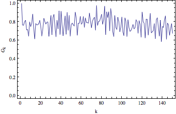
2nd Difference

	Autocorrelation	Partial Autocorrelation
Crime Series
1st Difference
2nd Difference

It looks like taking the first difference will produce a more stationary time series. The large negative autocorrelation at lag 1 in both the Acf and PAcf plot suggests the data may be better described with a moving average model component rather than with just an autoregressive model. Looks like it is bullocks on me for jumping the gun. I'll be back next post with a moving average model made in Mathematica. Until then, have fun with the source files for this post here.